MATLAB TUTORIAL 2- MATHEMATICAL FUNCTIONS AND BASIC CURVE PLOTTING

Hi friends its our second MATLAB tutorial and this time we are going to discuss  about  mathematical functions and basic curve plotting in MATLAB. MATLAB provides us a lot of commands and operation to deal with complex mathematical calculations and curve plotting….lets start….!!

MATHEMATICAL OPERATIONS

MATLAB provides us a lot of mathematical functions for computational purpose. There are a lot of predefined mathematical functions in MATLAB , you can get help about these functions by typing…

>> help elfun

For elementary functions and

>>help specfun

For special functions

This is the list of most commonly used mathematical functions

 x  is a variable of our choice.

These functions are built in MATLAB and also called as built- ins.

In addition to these functions MATLAB also provides us some predefined constant values . this table contains some predefined constant values

SOME EXERCISE

Let us suppose we have an expression to solve say

y=e2+sin(x)+log(z)        at x=5, z=6

So command will be

>> x=5;z=6;

>> y=exp(2)+sin(x)+log(z)

y =

      8.2219

Now suppose we have to solve

       x=sin(π/4)

Command will be

>> x=sin(pi/4)

x =

       0.7071

So now we are able to use all these functions for our calculation purpose but we have to be careful sometime as

1.      i and j which are generally defined as loop indices contains a constant value as iota in MATLAB so cannot be used as loop indices you have to use some other variables.

2.      Try to use built in functions on right hand side of the expression , reassigning the value can cause problem sometime.

CURVE PLOTTING

MATLAB has provided us a very powerful graphic tool set we can plot any function in 2D and in 3D too with the help of this tool set this time we are only focusing on 2D plotting have a look…

Simple plotting

Let us suppose we have to plot a curve between x and y with y=[1,4,5,7] at different values of x say x=[0,1,2,3] , now first of all we have to create linear array of x and y as

>>x=[0,1,2,3];

>>y=[1,4,5,7];

Then we can plot our graph using plot command as

>>plot(x,y)

Now on executing this command a window with corresponding plot will pop up as

Now suppose we have  to plot the graph of any function in a specified range say we have to plot graph of sin(x) in range x=[0 to 180]

So first of all we have to create a vector of x values ranging from 0 to 180 , then compute the sine of these values and finally plot it, command will be

>>x=0:pi/100:2*pi;                  (0means start at 0, pi/100 means increment of pi/100, stop at 180)                                       

>>y=sin(x);

>>plot(y)

And result will be

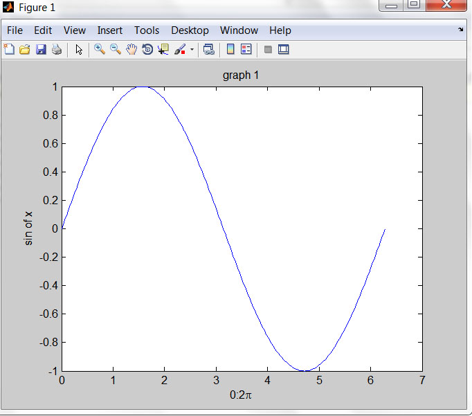
TITLES , LABLES AND ANNOTATIONS

We can also add titles , labels and annotations in plot , say in previous examples we have to add titles so commands will be

>>xlabel(‘0:2\pi’)                                  (here \pi creates chatacter π)

>>ylabel(‘sine of x’)

>>title(‘graph 1’)

And result will be

USING MULTIPLE DATA SETS ON A GRAPH

We can also plot more than one graph in a single plot, sat we have to plot two graphs as y1= sin(x), y2= cos(x)  for the range x= 0 to 2π

For this purpose commands will be

>>x=0:pi/100:2*pi;

>>y1=sin(x);

>>y2=cos(x);

>>plot(x,y1,’- -‘,x,y2,’-‘)

>>xlabel(‘0:2\pi’)

And finally result will be

LINE COLOUR ,STYLE AND MARKERS

For different plots and data sets we can use different line colour , styles and markers using the simple command

         plot(x,y,’style _colour_marker’)

here line_colour and marker is triplet from this table

you can find additional information by

>>help plot

Or

>> doc plot

so these are the basics of mathematics operations and plotting ...i hope this article was useful for you guys, in case of any query, doubt or critical view just leave a comment here...in our next tutorial we will discuss about basics of matrix and array.. till then bye....:)


     THNX